
1. Introduction to Linear Equations
Linear equations are everywhere. From predicting business profits to calculating distances, they form the backbone of mathematics and countless real-world applications. But what exactly are linear equations, and why do they matter?
At their core, linear equations represent a straight-line relationship between variables. They are simple yet powerful tools that help us understand patterns, make predictions, and solve complex problems efficiently. Whether you’re an IB student tackling algebra or a professional working with data, mastering linear equations is a fundamental skill.
What is a Linear Equation?
A linear equation is an equation that represents a straight line when graphed on a coordinate plane. It has the general form:
$$ax + b = 0$$
where:
- \(x\) is the variable
- \(a\) is the coefficient of \(x\) (a constant)
- \(b\) is a constant
In a two-variable system, a linear equation takes the form:
$$y = mx + c$$
where:
- \(y\) and \(x\) are variables
- \(m\) represents the slope (rate of change)
- \(c\) is the y-intercept (where the line crosses the y-axis)
Why Are Linear Equations Important?
Linear equations are crucial in various fields, including:
- Physics: Used to describe motion, force, and energy relationships.
- Economics: Helps in cost analysis, supply-demand models, and financial predictions.
- Engineering: Essential in circuit analysis, structural design, and mechanical modeling.
- Computer Science: Found in algorithms, data analysis, and artificial intelligence models.
They also play a key role in problem-solving, making them indispensable in daily life.
Basic Properties of Linear Equations
Linear equations share some key properties:
- They produce straight-line graphs.
- The degree (highest power of the variable) is always 1.
- They have a constant rate of change (slope).
- Solutions can be single values, infinite, or none (depending on the system).
2. Understanding Linear Equations
2.1 Definition of a Linear Equation
A linear equation is an algebraic equation in which each term is either a constant or the product of a constant and a single variable. These equations describe straight-line relationships and have no squared terms, cube roots, or higher-degree polynomials.
Key components include:
- Variables: Represent unknown quantities (e.g., \(x, y, z\)).
- Coefficients: Numbers multiplying variables (e.g., in \(5x\), the coefficient is 5).
- Constants: Fixed numbers without variables (e.g., 3, -7, 12).
Example Problem:
Let’s solve for \(x\) in the equation:
$$5x – 8 = 2$$
Step-by-Step Solution:
- Add 8 to both sides to isolate the \(5x\) term:
$$5x = 10$$
- Divide both sides by 5:
$$x = \frac{10}{5}$$
- Simplify:
$$x = 2$$
Thus, the solution is \(x = 2\).
2.2 The Graphical Meaning of a Linear Equation
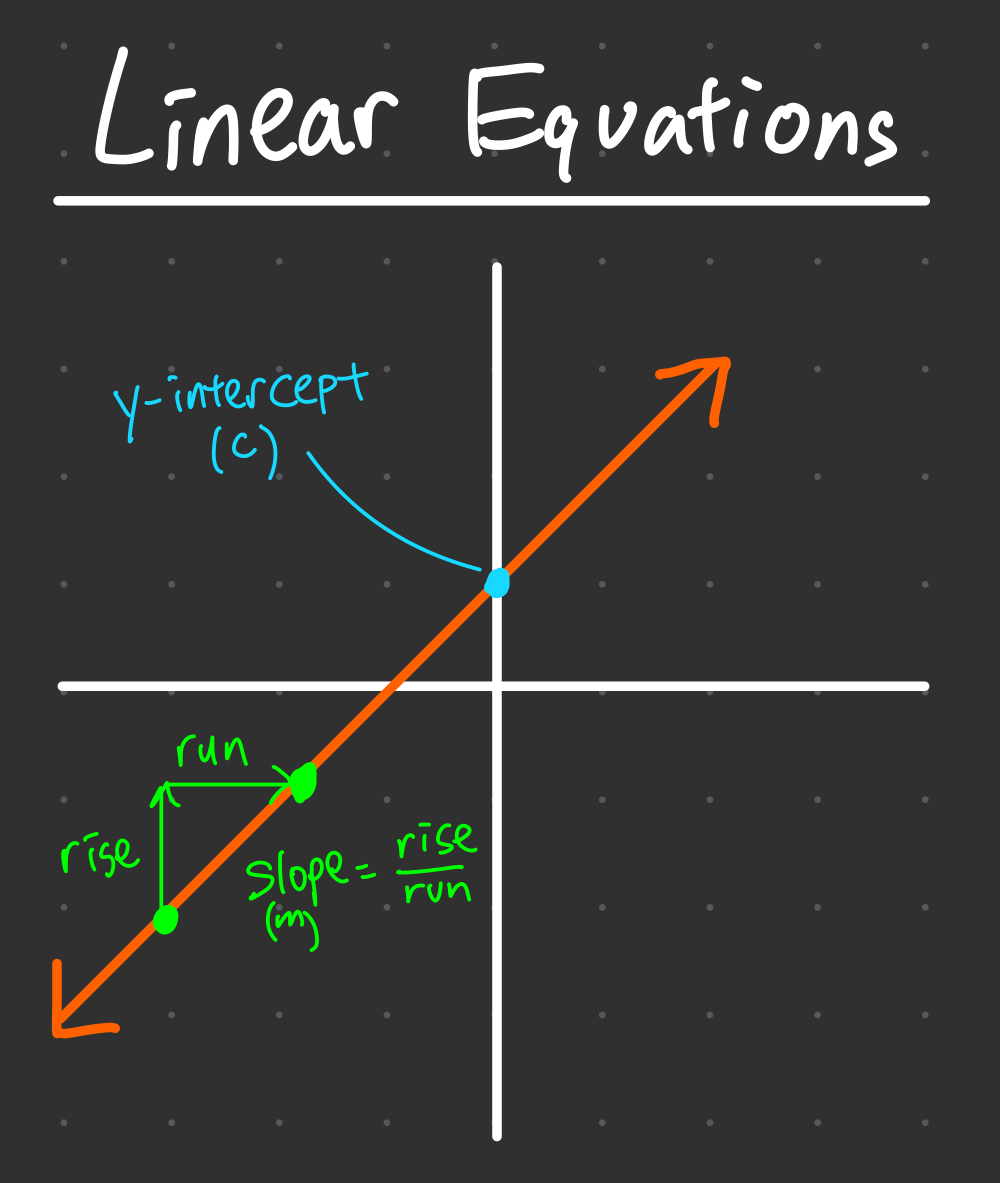
Linear equations, when plotted on a coordinate plane, always form straight lines. The equation \(y = mx + c\) defines a line with:
- \(m\) (Slope): Determines the steepness and direction of the line.
- \(c\) (Y-intercept): The point where the line crosses the y-axis.
Example Graphing:
Consider the equation:
$$y = 2x + 3$$
Key points:
- The slope \(m = 2\) means the line rises 2 units for every 1 unit it moves right.
- The y-intercept \(c = 3\) means the line crosses the y-axis at (0,3).
To plot the graph:
- Start at \( (0,3) \) on the y-axis.
- Use the slope: Move up 2 units and right 1 unit to get the next point.
- Draw a straight line passing through these points.
3. Forms of Linear Equations
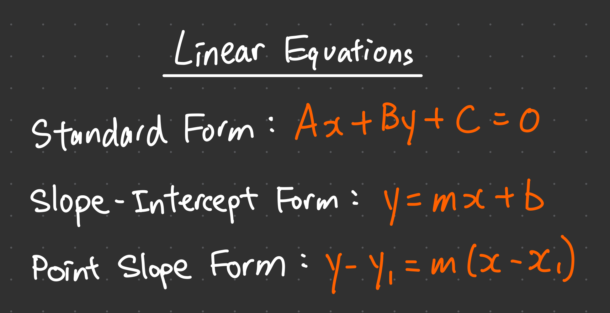
Linear equations can be written in different forms depending on the given information. The three most common forms are:
- Standard Form: \(Ax + By + C = 0\)
- Slope-Intercept Form: \(y = mx + b\)
- Point-Slope Form: \(y – y_1 = m(x – x_1)\)
Each form serves a unique purpose in algebra and real-world applications. Let’s explore them in detail.
3.1 Standard Form
The standard form of a linear equation is written as:
$$Ax + By + C = 0$$
where:
- \(A, B,\) and \(C\) are constants.
- \(x\) and \(y\) are variables.
- \(A\) and \(B\) cannot both be zero.
This form is useful for quickly identifying coefficients and for solving systems of equations using elimination.
Example: Convert \(4y = 2x + 10\) into Standard Form
Given equation:
$$4y = 2x + 10$$
Step-by-Step Conversion:
- Move all terms to one side:$$4y – 2x – 10 = 0$$
- Rearrange the terms in standard form:$$-2x + 4y – 10 = 0$$
- Multiply by \(-1\) to make the coefficient of \(x\) positive:$$2x – 4y + 10 = 0$$
Thus, the standard form of the equation is:
$$2x – 4y + 10 = 0$$
3.2 Slope-Intercept Form
The slope-intercept form is one of the most commonly used forms in algebra. It is written as:
$$y = mx + b$$
where:
- \(m\) is the slope of the line (rate of change).
- \(b\) is the y-intercept (where the line crosses the y-axis).
This form makes it easy to identify the slope and y-intercept, which helps in graphing and understanding how a line behaves.
Example: Identify the Slope and Intercept in \(y = -3x + 7\)
Given equation:
$$y = -3x + 7$$
- Slope (\(m\)): \(-3\), meaning the line decreases by 3 units for every 1 unit it moves right.
- Y-intercept (\(b\)): \(7\), meaning the line crosses the y-axis at (0,7).
Thus, the slope is \(-3\), and the y-intercept is \(7\).
3.3 Point-Slope Form
The point-slope form of a linear equation is written as:
$$y – y_1 = m(x – x_1)$$
where:
- \((x_1, y_1)\) is a given point on the line.
- \(m\) is the slope of the line.
This form is useful when you know one point and the slope but need to find the equation of the line.
Example: Find the Equation of a Line Passing Through (2,5) with a Slope of -4
We are given:
- Point: \( (2,5) \)
- Slope: \( m = -4 \)
Step-by-Step Solution:
- Use the point-slope formula:$$y – 5 = -4(x – 2)$$
- Distribute the slope:$$y – 5 = -4x + 8$$
- Add 5 to both sides:$$y = -4x + 13$$
Thus, the equation of the line is:
$$y = -4x + 13$$
4. How to Solve Linear Equations
Solving linear equations is a fundamental skill in algebra that helps us find unknown values in mathematical expressions. The approach depends on the number of variables involved. Below, we explore step-by-step methods for solving linear equations in one, two, and three variables.
4.1 Solving Linear Equations in One Variable
Linear equations in one variable have only one unknown and can be solved by isolating the variable. The general form is:
$$ax + b = c$$
Step-by-Step Method:
- Eliminate constants by adding or subtracting on both sides.
- Isolate the variable by dividing or multiplying.
- Verify by substituting the solution back into the equation.
Example: Solve \( \frac{3x – 5}{2} = 4 \)
Step-by-Step Solution:
- Multiply both sides by 2 to eliminate the fraction:$$3x – 5 = 8$$
- Add 5 to both sides:$$3x = 13$$
- Divide by 3:$$x = \frac{13}{3}$$
Thus, the solution is \( x = \frac{13}{3} \).
4.2 Solving Linear Equations in Two Variables
Linear equations with two variables have the general form:
$$Ax + By = C$$
Since there are two unknowns, we need two equations to find a unique solution. This is called a system of linear equations.
Methods to Solve a System of Two Linear Equations:
- Substitution Method: Solve one equation for a variable and substitute into the other.
- Elimination Method: Add or subtract equations to eliminate a variable.
- Graphical Method: Plot both equations and find their intersection.
Example: Solve the system
$$2x + 3y = 12$$
$$4x – y = 5$$
Using the Substitution Method:
- Solve for \( y \) in the second equation:$$y = 4x – 5$$
- Substitute \( y = 4x – 5 \) into the first equation:$$2x + 3(4x – 5) = 12$$
- Expand:$$2x + 12x – 15 = 12$$
- Simplify:$$14x = 27$$
- Divide by 14:$$x = \frac{27}{14}$$
- Substituting \( x = \frac{27}{14} \) into \( y = 4x – 5 \):$$y = 4 \times \frac{27}{14} – 5$$$$y = \frac{108}{14} – 5$$$$y = \frac{38}{14}$$$$y = \frac{19}{7}$$
Thus, the solution is \( x = \frac{27}{14}, y = \frac{19}{7} \).
4.3 Solving Linear Equations in Three Variables
For three variables, we need a system of three equations:
$$Ax + By + Cz = D$$
These are solved using substitution, elimination, or matrices.
Example: Solve the System
$$x + y + z = 10$$
$$2x – y + 3z = 5$$
$$-x + 4y – z = 7$$
Using the Substitution Method:
- Solve the first equation for \( x \):$$x = 10 – y – z$$
- Substitute into the second equation:$$2(10 – y – z) – y + 3z = 5$$
- Expand:$$20 – 2y – 2z – y + 3z = 5$$
- Simplify:$$20 – 3y + z = 5$$
- Rearrange:$$z = 3y – 15$$
- Substituting \( z = 3y – 15 \) into the third equation:$$-x + 4y – (3y – 15) = 7$$
- Using \( x = 10 – y – z \), substitute:$$-(10 – y – (3y – 15)) + 4y – (3y – 15) = 7$$
- Solve for \( y \):$$10 – y – 3y + 15 + 4y – 3y + 15 = 7$$$$40 – 3y = 7$$$$3y = 33$$$$y = 11$$
- Substituting \( y = 11 \) into \( z = 3y – 15 \):$$z = 3(11) – 15 = 18$$
- Using \( x = 10 – y – z \):$$x = 10 – 11 – 18$$$$x = -19$$
Thus, the solution is \( x = -19, y = 11, z = 18 \).
5. Real-World Applications of Linear Equations
Linear equations are not just theoretical concepts; they are used extensively in various fields to model real-world scenarios. From business to engineering, linear equations help professionals make predictions, optimize solutions, and solve practical problems. Let’s explore some key applications of linear equations in different domains:
Business: Calculating Profit and Expenses
In business, linear equations are often used to calculate profit, expenses, and revenue. For example, businesses track their income and costs using linear equations to make data-driven decisions and predict future financial performance.
For instance, consider a company that sells a product for $20 per unit and has fixed costs of $200. The total revenue can be modeled using a linear equation.
Example: A Company Sells a Product for $20 per Unit with Fixed Costs of $200. Write a Linear Equation for Total Revenue and Find the Break-Even Point.
Let:
- Revenue per unit sold = $20
- Fixed costs = $200
- Let \( x \) be the number of units sold.
The total revenue \( R \) can be expressed as:
$$ R(x) = 20x $$
Now, the company’s total costs \( C \) include both fixed and variable costs. If the variable costs per unit are $10, the total costs can be expressed as:
$$ C(x) = 200 + 10x $$
The company reaches its break-even point when total revenue equals total costs, i.e., when \( R(x) = C(x) \).
Finding the Break-Even Point:
Set the total revenue equal to the total costs:
$$ 20x = 200 + 10x $$
Step-by-Step Solution:
- Subtract \(10x\) from both sides:$$10x = 200$$
- Divide both sides by 10:$$x = 20$$
Thus, the company breaks even when they sell 20 units. At this point, the total revenue equals the total costs, and no profit or loss is incurred.
Physics: Motion Equations with Constant Velocity
Linear equations are also widely used in physics, particularly in motion problems where the velocity is constant. These types of problems are modeled using linear equations to represent position, velocity, and time.
For example, if an object moves at a constant velocity, its position can be modeled using the equation:
$$d = vt + d_0$$
where:
- \( d \) is the distance traveled.
- \( v \) is the velocity (speed) of the object.
- \( t \) is the time elapsed.
- \( d_0 \) is the initial distance (starting position).
This equation is crucial in calculating how far an object will travel over a specific period, given its velocity and initial position.
Engineering: Designing Structures with Balanced Forces
In engineering, linear equations are used to model systems with balanced forces, such as the design of bridges, buildings, or other structures. Engineers use linear equations to ensure that forces in a structure balance out, preventing failures and optimizing performance.
For instance, when designing a beam, the force applied at different points needs to be considered. The sum of forces in a system can be represented by a linear equation:
$$ F_1 + F_2 + F_3 = 0 $$
where \( F_1, F_2, F_3 \) are the forces acting on the beam, and the sum of these forces equals zero when the system is in equilibrium. Engineers use these equations to calculate how materials will behave under different loads and conditions.
6. Practice Problems
Now that you have a solid understanding of linear equations and their applications, it’s time to practice. Below are some problems that will test your skills in solving linear equations and working with different forms of linear equations. Try to solve them step-by-step and apply the methods you’ve learned.
Problem 1: Solve \( 7x + 2 = 3x + 10 \)
This is a linear equation in one variable. The goal is to isolate \( x \) on one side of the equation.
Step-by-Step Solution:
- Start by subtracting \( 3x \) from both sides:$$ 7x – 3x + 2 = 10 $$$$ 4x + 2 = 10 $$
- Next, subtract 2 from both sides:$$ 4x = 8 $$
- Now, divide both sides by 4:$$ x = 2 $$
The solution is \( x = 2 \).
Problem 2: Convert \( 5y = -2x + 15 \) to Standard Form
The standard form of a linear equation is \( Ax + By = C \). To convert this equation, we need to move all variables to one side and the constant to the other side.
Step-by-Step Solution:
- Start with the given equation:$$ 5y = -2x + 15 $$
- Move \( -2x \) to the left side by adding \( 2x \) to both sides:$$ 2x + 5y = 15 $$
The equation in standard form is \( 2x + 5y = 15 \).
Problem 3: Find the Equation of a Line Passing Through \( (4, -2) \) with a Slope of \( \frac{1}{2} \)
To find the equation of a line, we can use the point-slope form of a linear equation, which is:
$$ y – y_1 = m(x – x_1) $$
Where \( (x_1, y_1) \) is a point on the line, and \( m \) is the slope. In this case, the point is \( (4, -2) \) and the slope \( m = \frac{1}{2} \).
Step-by-Step Solution:
- Start with the point-slope form:$$ y – (-2) = \frac{1}{2}(x – 4) $$
- Simplify the equation:$$ y + 2 = \frac{1}{2}(x – 4) $$
- Distribute \( \frac{1}{2} \) on the right side:$$ y + 2 = \frac{1}{2}x – 2 $$
- Subtract 2 from both sides to solve for \( y \):$$ y = \frac{1}{2}x – 4 $$
The equation of the line is \(y = \frac{1}{2}x – 4\).
Problem 4: Solve the System of Equations:
$$3x + 2y = 14$$
$$x – y = 4$$
This is a system of two linear equations. You can solve this system using substitution, elimination, or graphical methods. Let’s use the substitution method here.
Step-by-Step Solution:
- Start by solving the second equation for \( x \):$$ x = y + 4 $$
- Substitute \( x = y + 4 \) into the first equation:$$ 3(y + 4) + 2y = 14 $$
- Expand and simplify:$$ 3y + 12 + 2y = 14 $$$$ 5y + 12 = 14 $$
- Subtract 12 from both sides:$$5y = 2$$
- Divide both sides by 5:$$y = \frac{2}{5}$$
- Substitute \( y = \frac{2}{5} \) back into \( x = y + 4 \):$$x = \frac{2}{5} + 4$$$$x = \frac{2}{5} + \frac{20}{5} = \frac{22}{5}$$
The solution to the system is \( x = \frac{22}{5}, y = \frac{2}{5} \).
7. Conclusion and Key Takeaways
In conclusion, linear equations are a fundamental concept in mathematics with a wide range of real-world applications. Understanding the different forms of linear equations—such as the standard form, slope-intercept form, and point-slope form—lays the foundation for solving a variety of problems, from business calculations to engineering designs and physics motion equations.
Recap of Different Forms of Linear Equations
Throughout this article, we explored the three primary forms of linear equations:
- Standard Form: \( Ax + By = C \), where \( A, B, C \) are constants, and \( x \) and \( y \) are variables.
- Slope-Intercept Form: \( y = mx + b \), where \( m \) is the slope of the line, and \( b \) is the y-intercept.
- Point-Slope Form: \( y – y_1 = m(x – x_1) \), where \( m \) is the slope and \( (x_1, y_1) \) is a specific point on the line.
Each form has its own advantages depending on the situation, making it crucial to understand when and how to use them effectively.
Importance of Understanding Solving Methods
Mastering the different methods for solving linear equations is equally important. Whether solving a single-variable equation or a system of equations with multiple variables, these techniques enable you to model and solve real-life problems. The ability to choose the appropriate method—such as substitution, elimination, or graphing—enhances your problem-solving skills and prepares you for more advanced topics in algebra and beyond.
Encouragement to Practice for Mastery
While the concepts and methods outlined here may seem challenging at first, the key to mastering linear equations is consistent practice. As you work through more problems, you’ll gain a deeper understanding of how to apply these principles in various contexts. Keep solving equations, exploring new problems, and testing your knowledge, and soon you’ll find that linear equations are no longer just an abstract concept but a powerful tool in your mathematical toolbox.
Remember, the more you practice, the more confident you will become in your ability to solve linear equations and apply them to real-world scenarios. Keep practicing, and the mastery of linear equations will soon be within your grasp!
Frequently Asked Questions (FAQ)
A linear equation is an algebraic equation in which the highest power of the variable(s) is 1. It represents a straight line when graphed and follows the general form \( Ax + By + C = 0 \) or \( y = mx + b \).
The three primary forms of linear equations are:
- Standard Form: \( Ax + By = C \)
- Slope-Intercept Form: \( y = mx + b \)
- Point-Slope Form: \( y – y_1 = m(x – x_1) \)
Each form is useful depending on the given information and the type of problem being solved.
The slope of a line, represented by \( m \), is calculated as the ratio of the change in \( y \)-values to the change in \( x \)-values between two points on the line:
$$ m = \frac{y_2 – y_1}{x_2 – x_1} $$
The slope indicates the steepness of the line: a positive slope rises from left to right, while a negative slope falls from left to right.
A linear equation forms a straight line when graphed and follows the general formula \( Ax + By = C \). A nonlinear equation, on the other hand, includes exponents higher than 1, variables multiplied together, or other operations that cause the graph to curve instead of forming a straight line.
There are three common methods to solve a system of linear equations:
- Substitution Method: Solve one equation for one variable and substitute it into the other equation.
- Elimination Method: Add or subtract equations to eliminate one variable and solve for the other.
- Graphical Method: Plot both equations on a graph and identify the point of intersection.
Linear equations are used in various real-world scenarios, including:
- Business: Calculating profit, expenses, and break-even points.
- Physics: Describing motion with constant velocity.
- Engineering: Designing stable structures and analyzing forces.
Linear equations are the foundation of algebra and essential in fields like science, economics, and engineering. They help solve real-world problems, make predictions, and understand relationships between variables. Mastering linear equations prepares you for more advanced mathematics and problem-solving in various disciplines.


